Theory of GNNs - Machine Learning with Graphs

Graph Isomorphism: It’s Harder Than It Looks¶

Definition: Two graphs $G$ and $H$ are isomorphic (iso: equal/same, morph: form/shape) if there exists a matching between their vertices so that two vertices are connected by an edge in $H$ if and only if corresponding vertices are connected by an edge in $G$ .

Optional Warm-Up: Play the following game for a few rounds: Isomorphism Game (Credit: Eric Mickelsen). Hint: You can move the nodes around.

Consider the following graphs $G$ and $H$ :

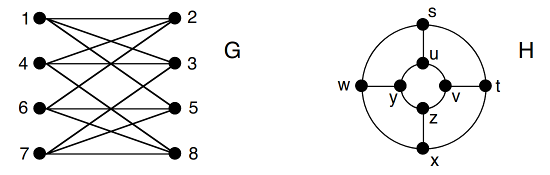
You are asked to check if these graphs are isomorphic or not. Find a mapping from nodes of $G$ to nodes of $H$ so that the structure is preserved.

At first glance, graph isomorphism may look simple: just “match the nodes”. However, as you can see, even for small graphs, finding an isomorphic mapping is not straightforward. For reference, in a protein-protein interaction (PPI) graph of the “simple” Escherichia Coli K12 bacterium, there are $\approx 4100$ nodes and $\approx 500000$ edges.
Now let’s think of the most naive approach to check if two given graphs are isomorphic. How many different matchings we need to check between two $n$ -node graphs in the worst case?

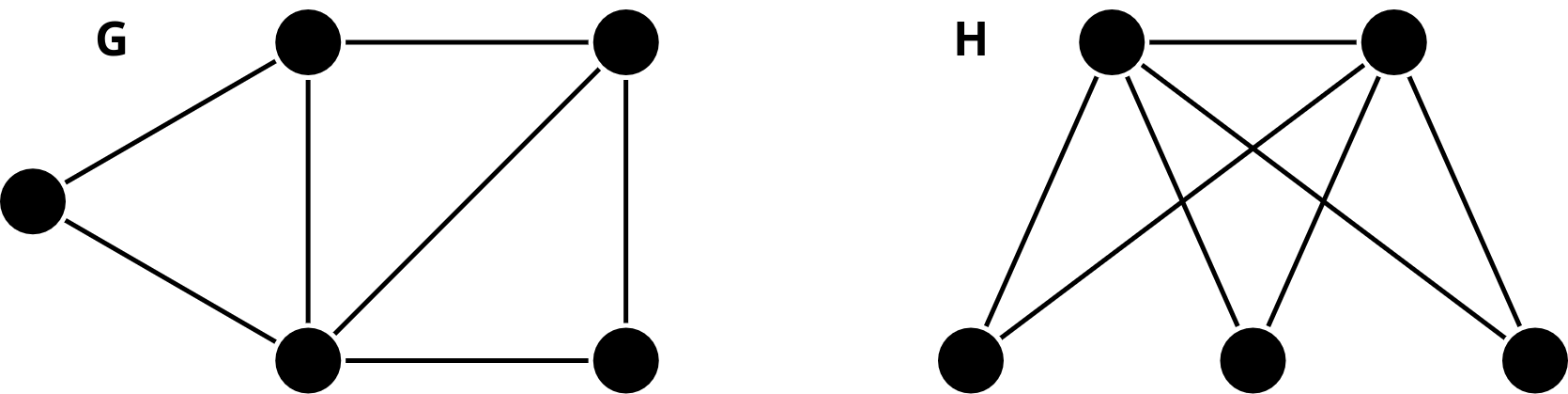
Let’s run a very simple GNN on these graphs:
$h_v^{(l)} = \sigma \left( W^{(l)} \sum_{u \in N(v)} \frac{h_u^{(l-1)}}{|N(v)|} \right)$
(1)
where $W=I$ (identity matrix), $\sigma$ is ReLU and all the nodes have the same initial feature vector $(1,1)^\top$ .
Compute the embeddings of node 1 in graph $G$ and node $s$ in graph $H$ after one iteration of message passing. Are they the same?

Based on (3) and the structure of both graphs, infer the graph-level embeddings of $G$ and $H$ obtained with mean-pooling (i.e., we take the average of all node embeddings in the graph). Are they the same?

Same graph-level embeddings mean that the GNN we used cannot distinguish isomorphic graphs. Is this a problem or a desirable property?

The Weisfeiler-Lehman Isomorphism Test¶

Luckily, brute-force checking of node labelings is not the only way to test if two graphs are isomorphic or not. Although it’s not perfect, the Weisfeiler-Lehman (WL) test is an efficient heuristic.

Initialization: Assign all nodes an initial label (e.g., 1).
Iteration: For each node $v$ :
1. Collect labels of all neighbors.
2. Form a multiset with its own label.
3. Hash this multiset into a new label for the node
Check convergence: Stop if labels don’t change, otherwise repeat.
Compare graphs: Collect the multiset of final node labels for each graph. If the multisets differ, then graphs are non-isomorphic. If identical → 1-WL cannot distinguish them.

Consider the following graphs $G$ and $H$ :

Tasks:

Apply WL test to determine if $G$ and $H$ are isomorphic or not. You can check this link for an example.

Multisets and Injectivity¶

Consider the following multisets:

$M_1 = \{ 1,3 \}$
$M_2 = \{ 1,1,3,3 \}$
$M_3 = \{ 1,1,1,1,1 \}$
$M_4 = \{ 2,3 \}$

Show that none of MEAN, MAX and SUM is injective over these multisets.
What about $\sum_{m\in M}2^m$ ?
What about $\sum_{m\in M}e^m$ ?
What’s the reason that $\sum_{m\in M}2^m$ produces collisions but $\sum_{m\in M}e^m$ does not?

Programming: Expressivity of GNNs, GCN vs GraphSAGE vs GIN¶

In this exercise, you will empirically investigate the expressive power of three Graph Neural Networks:

GCN (Kipf & Welling)
GraphSAGE (mean aggregator)
GIN (Graph Isomorphism Network)

You will compare how these architectures process two small graphs and analyze whether they can distinguish different structural roles of nodes. The graphs $G$ and $H$ are given in the following.

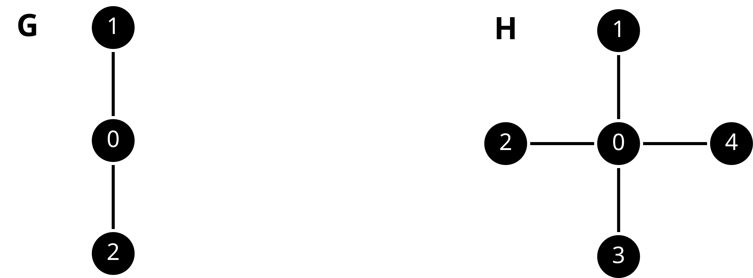
We assume that all nodes have the same feature vector $[1]$ .

First, let’s construct $G$ and $H$ in PyG.

import torch
from torch_geometric.data import Data

# Graph G: 3-node path (1 - 0 - 2)
g_edge_index = torch.tensor([
    [0,1,0,2],
    [1,0,2,0]
], dtype=torch.long)
g_x = torch.tensor([[1], [1], [1]], dtype=torch.float) # all features = 1
data_g = Data(x=g_x, edge_index=g_edge_index)

# Graph H: diamond graph
h_edge_index = torch.tensor([
    [0,1,0,2,0,3,0,4],
    [1,0,2,0,3,0,4,0]
], dtype=torch.long)
h_x = torch.tensor([[1], [1], [1], [1], [1]], dtype=torch.float) # all features = 1
data_h = Data(x=h_x, edge_index=h_edge_index)

Next, we’ll use the following implementations for GCN, GraphSAGE and GIN.

import torch.nn.functional as F
from torch_geometric.nn import GCNConv, SAGEConv, GINConv

class GCN(torch.nn.Module):
    def __init__(self, in_channels, hidden_channels, out_channels):
        super().__init__()
        self.conv1 = GCNConv(in_channels, hidden_channels)
        self.conv2 = GCNConv(hidden_channels, out_channels)

    def forward(self, x, edge_index):
        x = F.relu(self.conv1(x, edge_index))
        x = self.conv2(x, edge_index)
        return x

class GraphSAGE(torch.nn.Module):
    def __init__(self, in_channels, hidden_channels, out_channels):
        super().__init__()
        self.conv1 = SAGEConv(in_channels, hidden_channels, aggr='mean')
        self.conv2 = SAGEConv(hidden_channels, out_channels, aggr='mean')

    def forward(self, x, edge_index):
        x = F.relu(self.conv1(x, edge_index))
        x = self.conv2(x, edge_index)
        return x

class GIN(torch.nn.Module):
    def __init__(self, in_channels, hidden_channels, out_channels):
        super().__init__()
        nn1 = torch.nn.Sequential(
            torch.nn.Linear(in_channels, hidden_channels),
            torch.nn.ReLU(),
            torch.nn.Linear(hidden_channels, hidden_channels)
        )
        nn2 = torch.nn.Sequential(
            torch.nn.Linear(hidden_channels, hidden_channels),
            torch.nn.ReLU(),
            torch.nn.Linear(hidden_channels, out_channels)
        )
        self.conv1 = GINConv(nn1)
        self.conv2 = GINConv(nn2)

    def forward(self, x, edge_index):
        x = F.relu(self.conv1(x, edge_index))
        x = self.conv2(x, edge_index)
        return x

Now, let’s run one forward pass to see how the node embeddings change:

models = {
    "GCN": GCN(1, 16, 2),
    "GraphSAGE": GraphSAGE(1, 16, 2),
    "GIN": GIN(1, 16, 2)
}

for name, model in models.items():
    model.eval()
    print(f"=== {name} ===")
    for label, data in zip(["G", "H"], [data_g, data_h]):
        with torch.no_grad():
            emb = model(data.x, data.edge_index)
        print(f"{label} node embeddings:\n{emb}\n")

Task: Analyze the results:

Which models distinguish the center node (0) from the leaves (1 and 2)?
Compare the embeddings of node 0 in graphs $G$ and $H$ . Which models produce noticeably different embeddings?
Why GraphSAGE with mean aggregation collapses all embeddings when features start identical? Would it change if we switch to max aggregation as given below?
SAGEConv(in_channels, hidden_channels, aggr='max')
GCN also uses mean aggregator, but it can distinguish the center node, how?
To distinguish $G$ and $H$ with GraphSAGE, which global pooling method would you use, why?