A General Perspective on Graph Neural Networks - Machine Learning with Graphs

General GNN Framework¶

Consider the following GNN layer:

h_v^{(l)} = \sigma \left( \operatorname{AGG}^{(l)} \left( \{\operatorname{MSG}^{(l)}(h_u^{(l-1)} \mid u \in N(v))\} \right) \right)

(1)

Explain the role of AGG and MSG components.
Why must AGG be permutation invariant?
What issue arises in this formulation? (Hint: Consider how node $v$ incorporates information about itself.)
How can we modify this equation to fix the issue in (3)?
Modify the layer so that self-information and neighbor-information are treated differently. Provide the updated equation. (Hint: You are not limited to a single trainable weight matrix.)

Depth of a GNN¶

Consider the following GNN layer:

h_v^{(l)} = \operatorname{CONCAT} \big( \operatorname{AGG} \big( \{ m_u^{(l)} \mid u \in N(v) \} \big), m_v^{(l)} \big)

(2)

where $m_u^{(l)}=\operatorname{MSG}^{(l)}(h_u^{(l-1)})$ are the messages from neighbors and $m_v^{(l)}=\operatorname{MSG}^{(l)}(h_v^{(l-1)})$ is the self-message.

Assume that the AGG is the SUM function, and the messages $m_u^{(l)}$ and $m_v^{(l)}$ are $d$ -dimensional vectors. What is the dimension of $h_v^{(l)}$ ?
Discuss potential issues or challenges this concatenation might introduce when stacking multiple GNN layers.
Suggest a technique to control the dimension after concatenation.
Now, assume that we change the layer definition so that the concatenated vector is fed to a $k$ -layer multi-layer perceptron (MLP) as given in the following:
$h_v^{(l)} = \operatorname{MLP} \big( \operatorname{CONCAT} \big( \operatorname{AGG} \big( \{ m_u^{(l)} \mid u \in N(v) \} \big), m_v^{(l)} \big) \big)$
(3)
If we stack $L$ such layers, what will be the total depth of the GNN?

Graph Convolutional Networks¶

Consider the layer definition of the GCN by Kipf & Welling (paper link):

h_v^{(l+1)} = \sigma\left( \sum_{u \in N(v) \cup \{v\}} \frac{1}{\sqrt{\tilde{d}_v \tilde{d}_u}} \, h_u^{(l)} W^{(l)} \right)

(4)

where $\tilde{d}_v$ is the degree of node $v$ in the augmented adjacency $\tilde{A} = A + I$ after adding self-loops.

Compared to the simple normalization factor $\frac{1}{|N(v)|}$ we have seen in the lecture (W4, slide 17), what could be the reason to have $\frac{1}{\sqrt{\tilde{d}_v \tilde{d}_u}}$ (symmetric normalization)?
How does the GCN process a node’s own message differently from its neighbors’ messages?
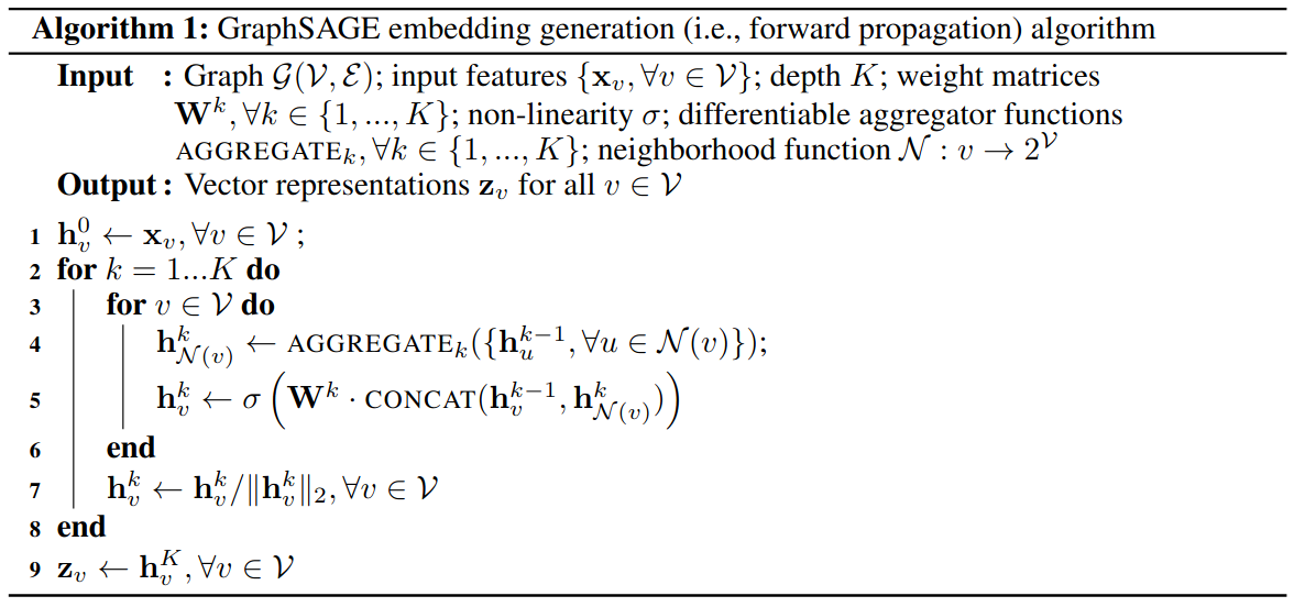
GraphSAGE (SAmple and aggreGatE) by Hamilton et. al. (paper link) is an extension of the GCN framework. Given the pseudocode below, list three aspects of GraphSAGE that is different from the original GCN and discuss how these changes improve the method.
How does the Graph Attention Network by Veličković et. al. (paper) improve the GCN?

Programming: Simple GNN with Torch¶

In this exercise, you’ll implement a simple GNN with pytorch and test on the Cora dataset (link).

The layer definition of the GNN you’ll implement is given as follows:

h_v^{(l)} = \sigma \left( W_{\text{self}}^{(l)} \cdot h_v^{(l-1)} + W_{\text{neigh}}^{(l)} \cdot \operatorname{AGG}^{(l)}\left(\{h_u^{(l-1)} \mid u \in N(v)\}\right) \right)

(5)

Basically, it uses two learnable weight matrices $W_{\text{self}}$ and $W_{\text{neigh}}$ that are multiplied with the messages from the node’s self and aggregated messages from neighbors, respectively. Then, the resulting vectors are summed and fed to $\sigma$ .

Complete the following code snippet given the following:
- Use MEAN aggretagor for neighbor messages.
- Use ReLU as $\sigma$ .

import torch
import torch.nn as nn
import torch.nn.functional as F

# A simple GNN layer that
# - aggregates neighbor features by mean
# - uses separate weight matrices for self and neighbor features
class SimpleGNNLayer(nn.Module):
    def __init__(self, in_dim, out_dim):
        super().__init__()
        self.linear_self = nn.Linear(in_dim, out_dim, bias=True)
        self.linear_neigh = nn.Linear(in_dim, out_dim, bias=True)

    def forward(self, x, edge_index):

        # edges j -> i (col = source, row = target)
        row, col = edge_index

        # messages are neighbor features
        messages = x[col]

        # aggregate by mean
        ############# your code here ############


    
        #########################################

        # update rule: combine self and neighbors with separate weights
        ############# your code here ############


    
        #########################################

        # return updated node features
        return out

# A simple 2-layer GNN model
class SimpleGNN(nn.Module):
    def __init__(self, in_dim, hidden_dim, out_dim):
        super().__init__()
        self.layer1 = SimpleGNNLayer(in_dim, hidden_dim)
        self.layer2 = SimpleGNNLayer(hidden_dim, out_dim)

    def forward(self, data):
        x, edge_index = data.x, data.edge_index

        # apply GNN layers with ReLU non-linearity
        ############# your code here ############


    
        #########################################

        return x

Now, train your GNN using the following script.

from torch_geometric.datasets import Planetoid

# load the Cora dataset
dataset = Planetoid(root='/tmp/Cora', name='Cora')

# model, data, optimizer
device = torch.device('cuda' if torch.cuda.is_available() else 'cpu')
model = SimpleGNN(in_dim=dataset.num_node_features, hidden_dim=16, out_dim=dataset.num_classes).to(device)
data = dataset[0].to(device)
optimizer = torch.optim.Adam(model.parameters(), lr=0.01, weight_decay=5e-4)

# training loop
train_losses = []
model.train()
for epoch in range(50):
    
    optimizer.zero_grad()
    out = model(data)
    
    # training loss
    loss = F.cross_entropy(out[data.train_mask], data.y[data.train_mask])
    loss.backward()
    optimizer.step()
    train_losses.append(loss.item())
    print(f"Epoch {epoch}: Train Loss = {loss.item():.4f}")

# final eval
model.eval()

pred = model(data).argmax(dim=1)
correct = (pred[data.test_mask] == data.y[data.test_mask]).sum()
acc = int(correct) / int(data.test_mask.sum())

print(f"Test Accuracy: {acc:.4f}")

Now, modify the SimpleGNN class so that it takes the number of layers as input.

Now, train two GNNs, one with 2 layers and another with 16. Then, compare the Mean Average Distance (MAD) of the embeddings learned by the models using the given function.
- Mean Average Distance (MAD): Average pairwise Euclidean distance between node embeddings.

def get_mad(embeddings):

    # embeddings: [N, d]  (N nodes, d-dimensional embeddings)
    N = embeddings.size(0)

    # Normalize embeddings
    embeddings = F.normalize(embeddings, dim=1)

    # Compute all pairwise Euclidean distances → shape [N, N]
    dist_matrix = torch.cdist(embeddings, embeddings, p=2)

    # Average the distances over all distinct pairs
    mad_val = dist_matrix.sum() / (N * (N - 1))

    return mad_val.item()

Interpret the accuracy and MAD values of models with 2 and 16 layers.