Neural Networks

A simple neural network to regress a quadratic function

Show code cell content Hide code cell content

import numpy as np
import torch
import torch.nn as nn
import matplotlib.pyplot as plt

from tqdm import tqdm, trange
from torch.distributions.uniform import Uniform

torch.manual_seed(19)
np.random.seed(19)

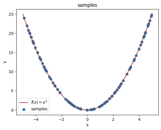
In this tutorial, we are investigating how a simple neural network approximates a simple non-linear function. In this case, we will try to approximate the quadratic function \(y = f(x) = x^2\):

# ground truth function f(x) = x^2 that we want to approximate
x_plot = np.linspace(-5, 5, 100)
y_plot = x_plot * x_plot

# draw training samples
x = np.random.uniform(-5, 5, 100)
y = x * x

def plot_samples(x, y, title = "samples"):
    global x_plot, y_plot
    plt.plot(x_plot, y_plot, color="tab:red", label="$f(x)=x^2$")
    plt.scatter(x, y, label="samples")
    plt.gca().set(xlabel="x", ylabel="y")
    plt.legend()
    plt.title(title)

plot_samples(x, y)

We will use PyTorch to build our neural network

from torch.optim import SGD

# number of hidden units
N_HIDDEN = 8

# define the layout of our neural network
model = nn.Sequential(
    nn.Linear(1, N_HIDDEN),
    # we will use ReLU as our non-linear activation function
    nn.ReLU(),
    nn.Linear(N_HIDDEN, 1)
)

# you can ignore this for now
# later, this hook will save as the latent representations
activations = dict()
def hook(module, x_in, x_out):
    global activations
    activations["latent"] = x_out.detach()
model[1].register_forward_hook(hook)

# the optimizer will update the model parameters for us
# we will use SGD: Stochastic Gradient Descent
LEARNING_RATE = 0.02
optimizer = SGD(model.parameters(), lr=LEARNING_RATE)

# number of iterations that we will train our model
EPOCHS = 5000

# our loss function: defines error between predictions and targets
# we will use Mean Squared Error, since it is a regression task
criterion = nn.MSELoss()

# for torch, we need to do some reshaping of our training data
# our network expects a single number as input
# so we need to reshape x/y from (100,) to (100,1), including a batch dimension
x_train = torch.from_numpy(x).reshape(-1, 1).float()
y_train = torch.from_numpy(y).reshape(-1, 1).float()

loss_log = []

for i in trange(EPOCHS):
    # 1. forward pass: get model predictions
    y_hat = model(x_train)
    # 2. compute loss: error between predictions and targets
    loss = criterion(y_hat, y_train)
    # 3. backward pass: propagate gradient trough network
    loss.backward()
    loss_log.append(loss.item())
    # 4. update parameters: perform one optimization step
    optimizer.step()
    # 5. reset torch gradients
    optimizer.zero_grad()

  0%|          | 0/5000 [00:00<?, ?it/s]

  6%|▌         | 280/5000 [00:00<00:01, 2796.76it/s]

 11%|█▏        | 563/5000 [00:00<00:01, 2812.19it/s]

 17%|█▋        | 849/5000 [00:00<00:01, 2831.51it/s]

 23%|██▎       | 1133/5000 [00:00<00:01, 2834.45it/s]

 28%|██▊       | 1417/5000 [00:00<00:01, 2832.11it/s]

 34%|███▍      | 1701/5000 [00:00<00:01, 2834.51it/s]

 40%|███▉      | 1986/5000 [00:00<00:01, 2836.81it/s]

 45%|████▌     | 2271/5000 [00:00<00:00, 2840.65it/s]

 51%|█████     | 2556/5000 [00:00<00:00, 2839.37it/s]

 57%|█████▋    | 2840/5000 [00:01<00:00, 2833.06it/s]

 62%|██████▎   | 3125/5000 [00:01<00:00, 2837.67it/s]

 68%|██████▊   | 3410/5000 [00:01<00:00, 2841.34it/s]

 74%|███████▍  | 3697/5000 [00:01<00:00, 2847.11it/s]

 80%|███████▉  | 3982/5000 [00:01<00:00, 2846.60it/s]

 85%|████████▌ | 4268/5000 [00:01<00:00, 2848.38it/s]

 91%|█████████ | 4553/5000 [00:01<00:00, 2848.29it/s]

 97%|█████████▋| 4839/5000 [00:01<00:00, 2849.82it/s]

100%|██████████| 5000/5000 [00:01<00:00, 2839.69it/s]

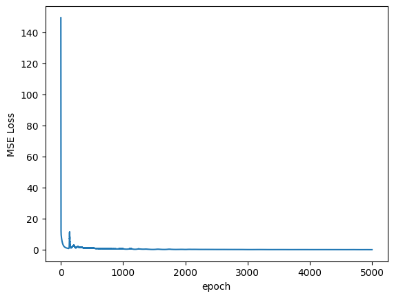
# plot the loss curve
plt.plot(loss_log)
plt.ylabel("MSE Loss")
plt.xlabel("epoch")

Text(0.5, 0, 'epoch')

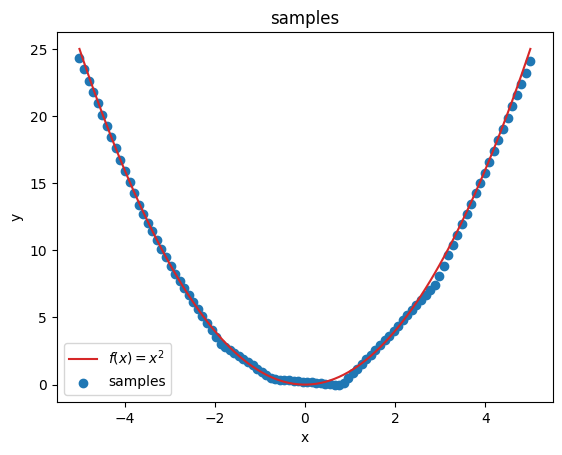
# don't need gradients to predict on whole linspace
with torch.no_grad():
    x_test = torch.from_numpy(x_plot).reshape(-1, 1).float()
    y_pred = model(x_test).reshape(-1).detach().numpy()

# plot predictions
plot_samples(x_plot, y_pred);

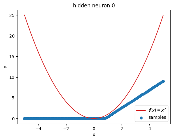
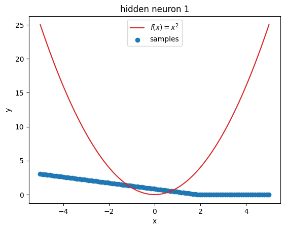
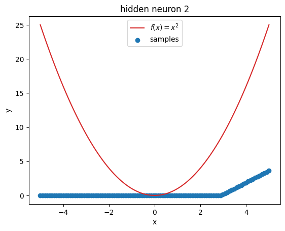
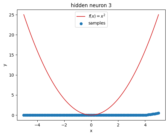
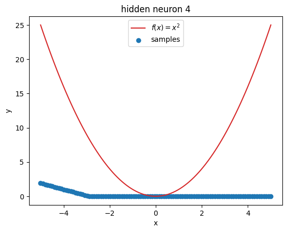
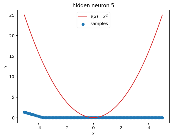
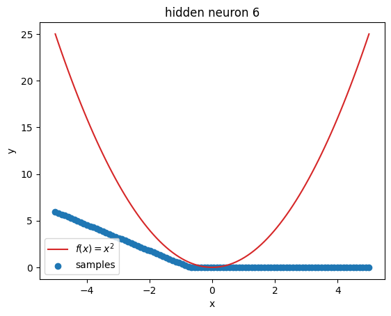
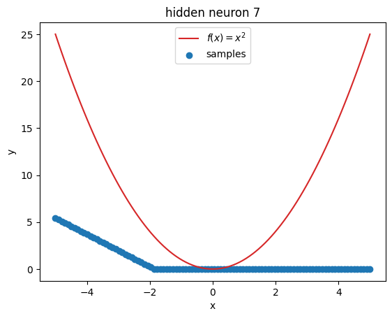
But what’s going on within the model? Let’s investigate by visualizing the latent activations. This gives us a clue, what each neuron learned:

z = activations["latent"]

for i in range(z.shape[1]):
    plt.figure()
    plot_samples(x_plot, z[:, i].detach().numpy(), f"hidden neuron {i}")

Prompts

1. Try out different values for LEARNING_RATE and EPOCHS. How does the loss change?

2. Try different numbers of hidden units by changing N_HIDDEN. How does the quality of the approximation change?

3. Head to the tensorflow playground (https://playground.tensorflow.org) and play around with network configurations!