Naive Bayes Classifier#
If it meows like a cat: A primer on Conditional Probabilities#
Let’s consider the probability:
What does this probability mean? From a frequentist point of view, probabilities just represent the expected relative number of observations. Therefore, \(p(cat) = 0.5\) only means, that a cat was observed \(50\%\) of the time. However, in Bayesian statistics, probabilities can be used to express beliefs about the world. Here, \(P(cat)\) could mean, that an observer is \(50\%\) sure, that the animal in front of him his a cat. This notion of representing beliefs instead of frequencies is useful, since it allows us to state our beliefs depending on the information that we have. Enter Conditional Probabilities, where the likelihood of observing event \(B\) after event \(A\) is denoted as:
For example, the probability of roling a \(6\) with a fair six-sided die is \(P(X = 6) = 1/6\). However, if another player already told us that the result is even, the probability changes to
Similarly, if the animal in front of us starts meowing, we might have a better idea, what kind of animal it actually is:
But how can we actually update our beliefs, once new information becomes available? This is described by Bayes Law, which can be derived from the definition of conditional probabilities:
In the context of a machine learning classifier, \(y\) could denote the class (e.g. “cat”), and \(x\) could denote an observerd feature of that class (e.g. “meows”). Our prior assumption is given by the prior \(p(y)\). It states our default belief of observing a certain class, without any other information about the observation \(x\) available. For example, if you have observed that there are 3 times as many dogs as cats on the world, your prior about observing a cat could be \(p(cat) = 0.25)\) and \(p(dog) = 0.75\). We want to update our prior belief with the information from observation \(x\) to obtain our posterior belief \(p(y | x)\), i.e. our belief after observing \(x\). Therefore, we multiply by the likelihood \(p(x | y)\), which describes, how likely that observation is, under the assumption, that we have a certain class \(y\) given. E.g., how likely is the animal to meow (\(x\)), if it is a cat (\(y\))? Seems pretty likely, doesn’t it? Finally, since probabilities should sum up to \(1\), if have to divide by the evidene \(p(x)\), i.e. the overall probability of observing \(x\). Sometimes, you will see the normalization term being omitted for classification, since
A Naive Bayes Classifier#
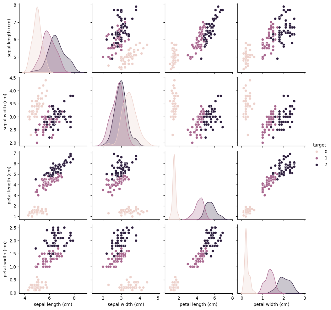
Enough with the theory already! Let’s look at a practical example. Consider the following dataset about cats and dogs:
Show code cell content
import numpy as np
import pandas as pd
import seaborn as sns
import matplotlib.pyplot as plt
import seaborn as sns

np.random.seed(19)
from sklearn.datasets import load_iris

iris_ds = load_iris()
X = iris_ds["data"]
y = iris_ds["target"]
feature_names = iris_ds["feature_names"]
iris_df = pd.DataFrame(X, columns=iris_ds["feature_names"])
iris_df["target"] = y
sns.pairplot(iris_df, hue = "target")
<seaborn.axisgrid.PairGrid at 0x7f98f04231a0>
Gaussian / Normal Distributions#
Probability Density Function (PDF):
def gaussian_pdf(x, loc=0, scale=1):
    # TODO
    pass
Show code cell content
def gaussian_pdf(x, loc=0, scale=1):
    norm = 1 / (scale * np.sqrt(2 * np.pi))
    p = -1 * np.power(x - loc, 2)
    q = 2 * np.power(scale, 2)
    return norm * np.exp(p / q)
class GaussianNaiveBayes:
    def __init__(self):
        self.loc_ = None
        self.scale_ = None
        self.priors_ = None
        self.classes_ = None
        self.feature_names_ = None

    def fit(self, X, y):
        self.classes_, self.priors_ = np.unique(y, return_counts=True)
        self.priors_ = self.priors_.astype(float) / len(y)
        _, p = X.shape
        self.loc_ = np.zeros(shape=(len(self.classes_), p))
        self.scale_ = np.zeros(shape=(len(self.classes_), p))
        for i, c in enumerate(self.classes_):
            self.loc_[i] = np.mean(X[y == c], axis=0)
            self.scale_[i] = np.std(X[y == c], axis=0)
        return self

    def predict(self, X):
        n, p = X.shape
        norm_probas = np.zeros(shape=(n, p, len(self.classes_)))
        for i, c in enumerate(self.classes_):
            norm_probas[:, :, i] = gaussian_pdf(X, self.loc_[i], self.scale_[i])
        # NAIVE Assumption: features are independent
        # compute likelihood by multiplying along feature axis
        likelihood = np.prod(norm_probas, axis=1)
        posterior = likelihood * self.priors_
        prediction = np.argmax(posterior, axis=1)
        return prediction
from matplotlib.patches import Ellipse
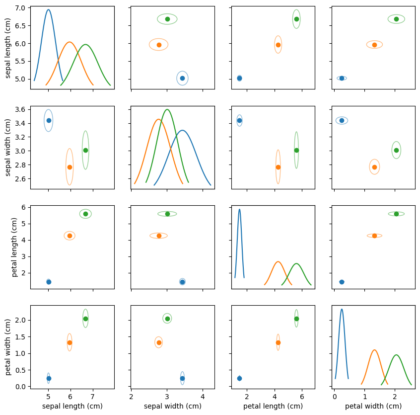
def plot_gnb(gnb):
# makeshift solution to get matching ellipse patch colors...
cycle = plt.rcParams['axes.prop_cycle'].by_key()['color']
c, p = gnb.loc_.shape
fig, axs = plt.subplots(p, p, figsize=(10,10), sharex="col", sharey="row")
for i in range(p):
for j in range(p):
if gnb.feature_names_:
if i == p - 1:
axs[i,j].set_xlabel(gnb.feature_names_[j])
if j == 0:
axs[i,j].set_ylabel(gnb.feature_names_[i])
if i == j:
loc = gnb.loc_[:, i]
scale = gnb.scale_[:, i]
x = np.linspace(loc - 2 * scale, loc + 2 * scale, 100)
y = gaussian_pdf(x, loc, scale)
axii = axs[i,i].twinx()
axii.set_yticks([])
for k, c in enumerate(gnb.classes_):
axii.plot(x[:,k], y[:,k], label=c)
else:
for k, c in enumerate(gnb.classes_):
loc_x = gnb.loc_[k, j]
loc_y = gnb.loc_[k, i]
axs[i,j].scatter(loc_x, loc_y, label=c)
std_patch = Ellipse((loc_x, loc_y), width=gnb.scale_[k,i], height=gnb.scale_[k,j], facecolor='none', edgecolor=cycle[k], alpha=0.5)
axs[i,j].add_patch(std_patch)
from sklearn.model_selection import train_test_split

X_train, X_test, y_train, y_test = train_test_split(X, y, random_state=19)

model = GaussianNaiveBayes()
model.fit(X_train, y_train)
model.feature_names_ = feature_names
plot_gnb(model)
from sklearn.metrics import accuracy_score

y_hat = model.predict(X_test)

accuracy_score(y_hat, y_test)
0.9210526315789473