t-SNE - DSC Tutorials

t-distributed Stochastic Neighbor Embedding

t-SNE: method to visualize high-dimensional data
not really for dimensionality reduction:
- non-deterministic projection into lower-dimensional space
- however, great for visualization
core idea: points that are neighbors in the high-dimensional space should still be neighbors in the low-dimensional space
van der Maaten and Hinton: Visualizing Data using t-SNE (2008)

import numpy as np
import pandas as pd
import seaborn as sns
import matplotlib.pyplot as plt
import scipy.stats as stats

from sklearn.datasets import make_classification
from sklearn.decomposition import PCA
from sklearn.manifold import TSNE
from tqdm import trange, tqdm

# for numeric stability
EPSILON = 10e-8

np.random.seed(19)
rng = np.random.default_rng(19)

Let’s start by creating a high-dimensional dataset, on which we can try t-SNE. We will use sklearn’s make_classification function, to create a dataset with 1000 samples, 50 features, and 2 classes. Of those 50 features, only 20 are informative, i.e., contain information about the class - the remaining 30 are random noise.

x_points, labels = make_classification(
    n_samples=1000,
    n_features=50,
    n_classes=2,
    n_informative=20,
    random_state=19
)

df = pd.DataFrame(x_points, columns=[f"x_{i}" for i in range(x_points.shape[1])])
df["label"] = labels
df.head()

If we plot the data and color each point by its class label, we might not necessarily see a difference between the 2 classes. Apparently, we picked 2 non-informative features, that are distributed identically in both classes.

sns.scatterplot(
    df,
    x="x_0",
    y="x_2",
    hue="label"
)

<Axes: xlabel='x_0', ylabel='x_2'>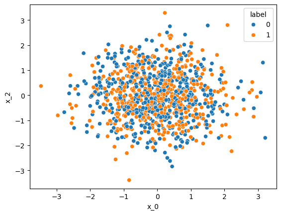

sns.boxplot(df, y="x_1", x="label")

<Axes: xlabel='label', ylabel='x_1'>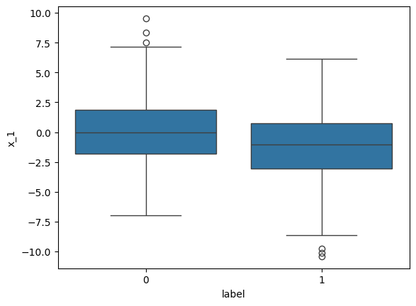

Now let’s try t-SNE: It will map all of the 50-dimensional points into a 2D space, so that we can visualize the points more efficiently:

from sklearn.manifold import TSNE

tsne = TSNE(n_components=2, random_state=19)

points_tsne = tsne.fit_transform(x_points)
points_tsne.shape

(1000, 2)

Now, if we visualize the 2D projection, we can see that blue points are closer to other blue points, while orange points also stick to themselves:

tsne_df = pd.DataFrame(points_tsne, columns=["tsne_1", "tsne_2"])
tsne_df["label"] = labels

sns.scatterplot(tsne_df, x="tsne_1", y="tsne_2", hue="label")

<Axes: xlabel='tsne_1', ylabel='tsne_2'>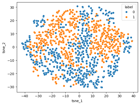

Let’s compare this with other dimensionality reduction techniques, e.g., PCA:

from sklearn.decomposition import PCA

pca = PCA(n_components=2)

points_pca = pca.fit_transform(x_points)
points_pca.shape

(1000, 2)

pca_df = pd.DataFrame(points_pca, columns=["pca_1", "pca_2"])
pca_df["label"] = labels

sns.scatterplot(pca_df, x="pca_1", y="pca_2", hue="label")

<Axes: xlabel='pca_1', ylabel='pca_2'>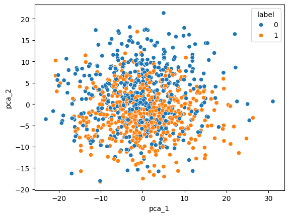

But how does it work?¶

The core idea of t-SNE is, that points that are neighbored in the high-dimensional space should also be neighbors in the low-dimensional space. More specifically, if points have a (relatively) low distance in the high-dimensional space, this should be reflected by their (relative) distance in the low-dimensional space.

How can we achieve that?

Using the pairwise distances between points in the high-dimensional space, we will define a probability distribution P: The conditional probability distribution $p_{j|i}$ , that point $i$ would select point $j$ as neighbor. This probability should be higher, the closer points $j$ and $i$ are.

Now, we can randomly initialize 2D coordinates that map the points into the lower-dimensional space. Again, we can compute a conditional probability distribution Q - this time based on the distances in the lower-dimensional space.

All we need to do now is to optimize the lower-dimensional (2D) coordinates, so that $Q$ is similar to $P$ . Therefore, we minimize the Kullback-Leibler Divergence between $P$ and $Q$ , which can be used to compute the distance between probability distributions.

Let’s start to implement t-SNE ourselves!

Implementing SNE¶

But before we look at t-SNE, let’s start with its predecessor: SNE. First, we need a function to compute pairwise Euclidean distances between points:

def get_delta(points_1, points_2):
    """
    Args:
        points_1: array of m points with shape (m, d) -> (m, 1, d)
        points_2: array of n points with shape (n, d)
    
    Returns:
        Array (m, n, d) that contains the pairwise differences between points_1 and points_2
    """
    # we will use numpy broadcasting to efficiently compute pairwise differences
    # differences: (m, 1, d) - (n, d) will be broadcasted to (m, n, d) 
    return points_1[:, np.newaxis, :] - points_2


def get_distance_matrix(points_1, points_2):
    """
    Computes a matrix that contains the pairwise distances between points_1 and points_2.

    Args:
        points_1: array of m points with shape (m, d) -> (m, 1, d)
        points_2: array of n points with shape (n, d)
    
    Returns:
        distance_matrixx:
            matrix of pairwise distances with shape (m, n, d)
            element m_{ij} contains euclidean distance between point i of points_1 and point j of points_2
    """ 
    delta = get_delta(points_1, points_2)
    # now we just need to 
    # could also use numpy.linalg.norm
    # from numpy.linalg import norm
    # distances = norm(differences, axis=2)

    # or we just implement the norm manually
    distances = np.sqrt(
        np.sum(delta * delta, axis=2)
    )

    return distances

# let's try if it works!
d = get_distance_matrix(x_points, x_points)

d.shape

(1000, 1000)

# the diagonal should contain only 0s since the distance of each point to itself is 0
np.all(np.diagonal(d) == 0)

np.True_

Next, we need to implement a function that computes the conditional probabilities as given in Equation (1) in the paper:

p_{j|i} = \frac{\exp[ - \lVert x_i - x_j \rVert^2 / 2 \sigma_i^2]}{ \sum_{k\neq i} \exp [- \lVert x_i - x_k \rVert^2 / 2 \sigma_i^2]}

(1)

We will ignore the variance term $\sigma$ for now - notice that we also don’t need it in the lower dimensional space:

q_{j|i} = \frac{\exp[ - \lVert y_i - y_j \rVert^2 ]}{ \sum_{k\neq i} \exp [- \lVert y_i - y_k \rVert^2 ]}

(2)

def get_conditional_probas(distances, sigma=None):
    """
    Conditional probabilities P in the higher dimensional space
    Implements Equation (1).

    Returns:
        M: numpy matrix, where m_{ij} is the conditional probability p_{j|i}
        Where i is the row index and j is the column index.
        I.e., each row is a conditional probability distribution, that adds up to 1.
    """
    if sigma is None:
        # don't use sigma, i.e., for the lower dimensional probability distribution
        exp_dists = np.exp(-1 * np.power(distances, 2))
    else:
        # expand sigma to broadcast over rows
        sigma = sigma[:, np.newaxis]
        exp_dists = np.exp(-1 * np.power(distances, 2) / (2 * np.power(sigma, 2)))

    # a little trick: we set diagonal elements to 0
    # since we want to exclude points where k==l
    np.fill_diagonal(exp_dists, 0)

    # use keepdims=True to divide row-wise, instead of column-wise
    q = exp_dists / exp_dists.sum(axis=1, keepdims=True)

    return q

# should NOT add up to 1 as each row represents a conditional probability distribution!
get_conditional_probas(d).sum()

np.float64(1000.0)

# instead, each row adds (roughly) up to 1
np.unique(
    get_conditional_probas(d).sum(axis=1)
)

array([1., 1., 1., 1., 1., 1.])

Now, let’s implement the cost function:

\tag{2} C_{SNE} = \sum_i \mathrm{KL}(P_i \Vert Q_i) = \sum_i \sum_j p_{j|i} \log\frac{p_{j|i}}{q_{j|i}}

(3)

Here, $\mathrm{KL(P_i \Vert Q_i)}$ is the Kullback-Leibler Divergence, which we want to minimize.

def get_sne_cost(p_probas, q_probas, mask_diagonal=True):
    """
    Implements Equation (2) of the paper. 
    """
    if mask_diagonal:
        # trick to avoid running into errors for diagonal with 0 elements
        p_probas = p_probas.copy()
        np.fill_diagonal(p_probas, 1)
        q_probas = q_probas.copy()
        np.fill_diagonal(q_probas, 1)
    
    pq_ratio = np.maximum(p_probas / np.maximum(q_probas, EPSILON), EPSILON)
    
    return np.sum(p_probas * np.log(pq_ratio))

Our objective is to get the Kullback-Leibler Divergence between the higher-dimensional and the lower-dimensional distribution as small as possible. Therefore, we will compute the gradient of the SNE cost function with regard to the lower-dimensional coordinates of each point. Then, we can use gradient descent to move the points around in the lower-dimensional space, until the Kullback-Leibler Divergence is minimal.

def get_sne_gradient(p_probas, q_probas, y_points):
    """
    Computes the gradient of the SNE cost function.
    """
    # shape (n, n, 1)
    pq = (p_probas - q_probas + p_probas.T - q_probas.T)[:, :, np.newaxis]
    # shape (n, n, y_ndim)
    y_delta = get_delta(y_points, y_points)
    # shape (n, y_ndim)
    return 2 * np.sum(pq * y_delta, axis=1)

Until now, we ignored the sigma term in the higher-dimensional probability distribution. Since it is the last missing piece, we have to talk about it now, unfortunately.

def get_entropy(probas, mask_diagonal=True):
    # earlier, we used a trick to set diagonal elements to 0
    # this will cause errors now, as log2(0) is not defined
    # we will use another trick, and set it to 1 now
    if mask_diagonal:
        probas = probas.copy()
        np.fill_diagonal(probas, 1)
     
    log_probas = np.log2(np.maximum(probas, EPSILON))
    return -np.sum(probas * log_probas, axis=1)

def get_perplexity(probas, mask_diagonal=True):
    return np.power(2, get_entropy(probas, mask_diagonal=mask_diagonal))

def get_sne_sigma(distances, perplexity=30, sigma_start=1, steps=30):
    """
    Implement binary search to get optimal sigmas.
    
    1. compute the probability matrix with start sigma
    2. compute perplexity from probability matrix
    3. optimize sigmas to get closer to target perplexity and repeat
    """
    target = perplexity
    n, m = distances.shape

    sigma = np.full(shape=(n), fill_value=sigma_start)
    sigma_low = np.zeros_like(sigma)

    for i in range(steps):
        sigma_mid = (sigma + sigma_low) / 2
        probas = get_conditional_probas(distances, sigma=sigma)
        perplexity = get_perplexity(probas, mask_diagonal=True)

        # optimize sigma via binary search
        # if perplexity is lower than target perplexity: increase sigma
        # because entropy and therefore perplexity increase with variance sigma
        sigma_low = np.where(perplexity < target, sigma, sigma_low)

        sigma = np.where(perplexity < target, 2 * sigma, sigma_mid)
    return sigma

We have everything we need now! Let’s put it all together and implement the SNE algorithm:

def get_sne(x_points, y_points=None, y_ndim=2, perplexity=30, steps=100, lr=0.01, log_frames=False, log_frame_interval=1):
    n, x_ndim = x_points.shape
    x_distances = get_distance_matrix(x_points, x_points)

    sigma = get_sne_sigma(x_distances, perplexity=perplexity)

    p_probas = get_conditional_probas(x_distances, sigma=sigma)

    if y_points is None:
        y_points = np.random.normal(size=(n, y_ndim))

    costs = []
    frames = []

    for i in trange(steps):
        if log_frames and i % log_frame_interval == 0:
            frames.append(y_points.copy())
        
        y_distances = get_distance_matrix(y_points, y_points)
        q_probas = get_conditional_probas(y_distances)

        cost = get_sne_cost(p_probas, q_probas, mask_diagonal=True)
        costs.append(cost)

        gradient = get_sne_gradient(p_probas, q_probas, y_points)

        # optimize the lower-dimensional coordinates via gradient-descent
        y_points -= lr * gradient
    
    result = {"costs": costs, "y_points": y_points}

    if log_frames:
        result["frames"] = frames

    return result

sne_result = get_sne(x_points, lr=10e-2, steps=100, perplexity=5)

sne_costs = sne_result["costs"]
sne_points = sne_result["y_points"]

sne_df = pd.DataFrame({
    "sne_1": sne_points[:, 0],
    "sne_2": sne_points[:, 1],
    "label": labels
})

  8%|▊         | 8/100 [00:00<00:06, 14.68it/s]

100%|██████████| 100/100 [00:06<00:00, 14.62it/s]

plt.plot(sne_result["costs"])
plt.title("SNE KL loss");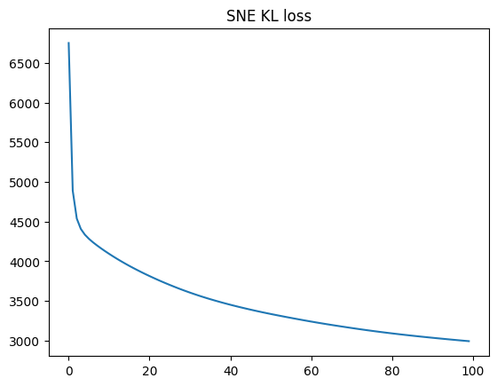

Let’s look at the SNE transformed points:

sns.scatterplot(sne_df, x="sne_1", y="sne_2", hue="label")
plt.title("SNE of make_classification");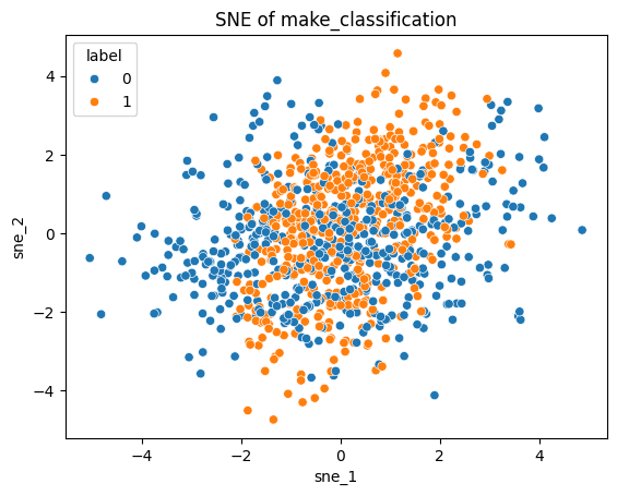

SNE of sklearn digits¶

Let’s try our SNE implementation on the digits dataset from sklearn.

from sklearn.datasets import load_digits

digits = load_digits()

plt.imshow(digits.images[0], cmap="gray");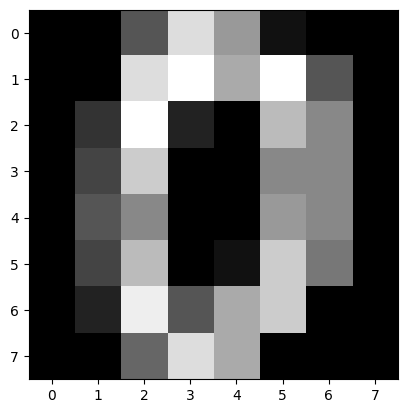

# this is how one "point" looks like
digits.data[0]

array([ 0.,  0.,  5., 13.,  9.,  1.,  0.,  0.,  0.,  0., 13., 15., 10.,
       15.,  5.,  0.,  0.,  3., 15.,  2.,  0., 11.,  8.,  0.,  0.,  4.,
       12.,  0.,  0.,  8.,  8.,  0.,  0.,  5.,  8.,  0.,  0.,  9.,  8.,
        0.,  0.,  4., 11.,  0.,  1., 12.,  7.,  0.,  0.,  2., 14.,  5.,
       10., 12.,  0.,  0.,  0.,  0.,  6., 13., 10.,  0.,  0.,  0.])

# each point is labeled as number from 0 to 9
digits.target

array([0, 1, 2, ..., 8, 9, 8], shape=(1797,))

from sklearn.preprocessing import MinMaxScaler

scaler = MinMaxScaler()

digits_n, digits_ndim = digits.data.shape

# scale, so that maximum distance is 1!
digit_points = scaler.fit_transform(digits.data) / np.sqrt(digits_ndim)

digit_labels = digits.target

digit_sne = get_sne(digit_points, lr=0.1, log_frames=True, log_frame_interval=1)

100%|██████████| 100/100 [00:24<00:00,  4.09it/s]

plt.plot(digit_sne["costs"])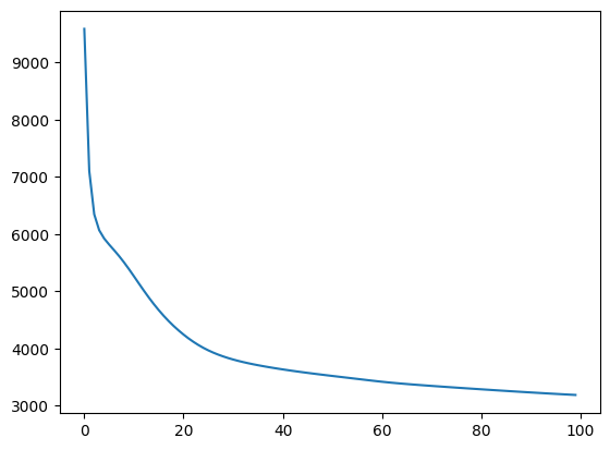

sne_digits_df = pd.DataFrame({
    "sne_1": digit_sne["y_points"][:, 0],
    "sne_2": digit_sne["y_points"][:, 1],
    "label": digit_labels.astype(str)
})

sns.scatterplot(sne_digits_df, x="sne_1", y="sne_2", hue="label")
plt.title("Digits SNE");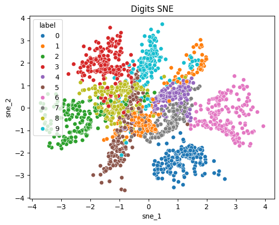

from IPython.display import HTML
from matplotlib.animation import FuncAnimation

def show_frames(frames, c=None, resize=True):
    fig, ax = plt.subplots()
    x = frames[0]
    scatter = ax.scatter(x[:, 0], x[:, 1], c=c)

    def update(frame):
        scatter.set_offsets(frame)
        if resize:
            xlim = np.abs(frame[:,0]).max() * 1.05
            ylim = np.abs(frame[:,1]).max() * 1.05
            ax.set_xlim(-xlim, xlim)
            ax.set_ylim(-ylim, ylim)
        return [scatter]
    
    anima = FuncAnimation(
        fig,
        update,
        frames=frames,
        interval=30,
        blit=True
    )

    # anima.save("sne.gif")

    plt.close(fig)
    
    return HTML(anima.to_jshtml())

digit_frames = digit_sne["frames"]

show_frames(digit_frames, c=digit_labels)

From SNE to t-SNE¶

So, we have a working implementation of SNE. However, van der Maaten and Hinton pointed out 2 issues with SNE:

Instead of a single KL Divergence, SNE actually minimizes the sum of KL Divergences between conditional probability distributions.
The “Crowding Problem”: Since we have a lot more volume in higher-dimensional spaces, accurately preserving pairwise distances in the lower-dimensional space is difficult. If we want to map points with small distances accurately, SNE tends to squeeze points with high-distances together at the center of the 2-dimensional map.

To adress those drawbacks of SNE, they proposed two modifications:

Instead of many conditional, t-SNE uses one symmetric probability distribution for the higher and lower dimensional space respectively.
Instead of a Gaussian distribution, they used a distribution with a heavy tail to model the neighborhoods in the lower-dimensional space. This stretches the lower-dimensional points out, solving the crowding problem. The heavy-tailed distribution they chose is the Student t-distribution - thus putting the t in t-SNE.

Making SNE symmetric¶

Following Section 3.1 of the paper, we need to modify how we compute the probability distributions a bit. Instead of conditional probability distributions $p_{j|i}$ , we want to consider symmetric joint probability distributions $p_{ij} = p_{ji}$ .

I.e., instead of having a probability of choosing point $j$ as neighbor given point $i$ , we now consider the probability of points $i$ and $j$ being neighbors.

Note that instead of each row adding up to 1, now the whole matrix should add up to 1.

In the lower-dimensional space, we will use this symmetric distribution:

\tag{3} q_{ij} = \frac{exp[-\lVert y_i - y_j \rVert^2]}{\sum_{k\neq\color{red} l}\exp [-\lVert y_k - y_{\color{red}l} \rVert^2]}

(4)

This looks very similar to the conditional distribution we used before - however, note how in the denominator, we are now computing the sum over all pairwises distances, not only the distances to the point we are conditioning on.

def get_joint_probas(distances, sigma=None):
    """
    Symmetrical probabilities Q in the lower dimensional space
    
    Implements Equation (3) of the paper.
    """
    if sigma is None:
        exp_dists = np.exp(-1 * np.power(distances, 2))
    else:
        sigma = sigma[:, np.newaxis]
        exp_dists = np.exp(-1 * np.power(distances, 2) / (2 * np.power(sigma, 2)))

    # a little trick: we set diagonal elements to 0
    # since we want to exclude points where k==l
    np.fill_diagonal(exp_dists, 0)

    q = exp_dists / exp_dists.sum()
    return q

# this should add up (roughly) to 1
get_joint_probas(d).sum()

np.float64(1.0)

However, in the high-dimensional space, they propose to symmetrize the conditional probability distributions $p_{j|i}$ and $p_{i|j}$ to avoid running into problems with outliers with no neighboring points:

def get_symmetric_probas(probas):
    """Symmetrizes a conditional probability distribution as given in section 3.1"""
    n, m = probas.shape

    if n != m:
        raise ValueError("probability matrix must be symmetric!")

    # divide by 2 n, to make sure that probability mass over all points adds up to 1
    probas =  (probas + probas.T) / (2*n)
    return probas

# should add up to 1 again
get_symmetric_probas(get_conditional_probas(d)).sum()

np.float64(1.0)

Putting the t in t-SNE¶

Fun Fact: The Student t-distribution is NOT named like that because it is used to irritate students. It was developed in 1908 by Willliam Sealy Gosset, who published it under his pseudonym “Student”.

# normal distribution vs Student t-distribution
import scipy.stats as stats

def plot_dists():
    x = np.linspace(-3, 3, 100)
    y_norm = stats.norm.pdf(x)

    plt.plot(x, y_norm, label="Gaussian N(0,1)", color="k", linestyle="--")

    for t in [2, 5, 10]:
        y_t = stats.t.pdf(x, t)
        plt.plot(x, y_t, label=f"Student's t({t})")

    plt.legend()
    plt.title("Gaussian vs Student's t Distribution")
    plt.xlabel("x")
    plt.ylabel("P(x)")

plot_dists()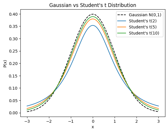

As you can see, the Student’s t distribution assigns more probability mass to extreme events than the standard normal distribution, which is what makes it “heavy-tailed”.

Although we could use the symmetric joint probability distribution in the lower dimensional space, they propose to use the Student’s t-distribution here to address the crowding problem:

\tag{4} q_{ij} = \frac{(1 + \lVert y_i - y_j \rVert^2)^{-1}}{\sum_{k\neq l} (1 + \lVert y_k - y_l \rVert^2)^-1}

(5)

def get_joint_t_probas(distances):
    t = 1 / (1 + np.power(distances, 2))

    # again, trick to mask out diagonal
    np.fill_diagonal(t, 0)

    return t / t.sum()

get_joint_t_probas(d).sum()

np.float64(1.0)

Assembling t-SNE¶

def get_tsne_cost(p_probas, q_probas, mask_diagonal=True):
    """
    Implements Equation (2) of the paper. 
    """
    if mask_diagonal:
        # trick to avoid running into errors for diagonal with 0 elements
        p_probas = p_probas.copy()
        np.fill_diagonal(p_probas, 1)
        q_probas = q_probas.copy()
        np.fill_diagonal(q_probas, 1)
    
    pq_ratio = np.maximum(p_probas / np.maximum(q_probas, EPSILON), EPSILON)
    
    return np.sum(p_probas * np.log(pq_ratio))

\tag{5} \frac{\partial C}{\partial y_i} = 4\sum_j (p_{ij} - q_{ij}) (y_i - y_j) (1 + \lVert y_i - y_j \rVert^2)^{-1}

(6)

def get_tsne_gradient(p_probas, q_probas, y_points):
    """
    Args:
        p (n,n)
        q (n,n)
        y (n,d_{lower})
    
    Results:
        g (n, d)
    """
    # compute differences
    y_delta = get_delta(y_points, y_points)

    # shape (n,n,1)
    pq_delta = (p_probas - q_probas)[:, :, np.newaxis]

    # shape (n, n, 1)
    distances = get_distance_matrix(y_points, y_points)[:, :, np.newaxis]

    # shape (n,n,1)
    t = 1 / (1 + np.power(distances, 2))

    return 4 * (pq_delta * y_delta * t).sum(axis=1)

def get_tsne_sigma(distances, perplexity=30, sigma_start=1, steps=30):
    """
    Implement binary search to get optimal sigmas.
    
    1. compute the probability matrix with start sigma
    2. compute perplexity from probability matrix
    3. optimize sigmas to get closer to target perplexity and repeat
    """
    target = perplexity
    n, m = distances.shape

    sigma = np.full(shape=(n), fill_value=sigma_start)
    sigma_low = np.zeros_like(sigma)

    for i in range(steps):
        sigma_mid = (sigma + sigma_low) / 2

        # use symmetric probas instead
        conditionals = get_conditional_probas(distances, sigma=sigma)
        probas = get_symmetric_probas(conditionals)

        perplexity = get_perplexity(probas, mask_diagonal=True)

        # optimize sigma via binary search
        # if perplexity is lower than target perplexity: increase sigma
        # because entropy and therefore perplexity increase with variance sigma
        sigma_low = np.where(perplexity < target, sigma, sigma_low)

        sigma = np.where(perplexity < target, 2 * sigma, sigma_mid)
    return sigma

The number of gradient descent iterations T was set 1000, and the momentum term was set to α(t) = 0.5 for t < 250 and α(t) = 0.8 for t ≥ 250. The learning rate η is initially set to 100 and it is updated after every iteration by means of the adaptive learning rate scheme described by Jacobs (1988).

def get_momentum(t):
    if t < 250:
        return 0.5
    return 0.8

def get_tsne(x_points, y_points=None, y_ndim=2, perplexity=30, steps=1000, lr=100, log_frames=False, log_frame_interval=1):
    n, x_ndim = x_points.shape
    x_distances = get_distance_matrix(x_points, x_points)

    # use symmetric probabilities to compute sigma
    # sigma = get_tsne_sigma(x_distances, perplexity=perplexity)
    sigma = get_sne_sigma(x_distances, perplexity=perplexity)

    # use symmetric joint probabilities for high-dimensional space
    p_conditionals = get_conditional_probas(x_distances, sigma=sigma)
    p_probas =  get_symmetric_probas(p_conditionals)

    if y_points is None:
        y_points = rng.normal(size=(n, y_ndim))

    costs = []
    frames = []
    y_delta = 0

    for i in trange(steps):
        if log_frames and i % log_frame_interval == 0:
            frames.append(y_points.copy())
        
        y_distances = get_distance_matrix(y_points, y_points)

        # use joint t-distribution for lower-dimensional space
        q_probas = get_joint_t_probas(y_distances)

        cost = get_tsne_cost(p_probas, q_probas, mask_diagonal=True)
        costs.append(cost)

        gradient = get_tsne_gradient(p_probas, q_probas, y_points)

        # optimize the lower-dimensional coordinates via gradient-descent
        momentum = get_momentum(i) 
        y_delta = -lr * gradient + momentum * y_delta
        y_points += y_delta
    
    result = {"costs": costs, "y_points": y_points}

    if log_frames:
        result["frames"] = frames

    return result

tsne_result = get_tsne(x_points)

tsne_costs = tsne_result["costs"]
tsne_points = tsne_result["y_points"]

tsne_df = pd.DataFrame({
    "tsne_1": tsne_points[:, 0],
    "tsne_2": tsne_points[:, 1],
    "label": labels
})

100%|██████████| 1000/1000 [01:39<00:00, 10.10it/s]

plt.plot(tsne_result["costs"])
plt.title("t-SNE KL loss");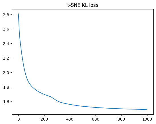

sns.scatterplot(tsne_df, x="tsne_1", y="tsne_2", hue="label")
plt.title("t-SNE of make_classification");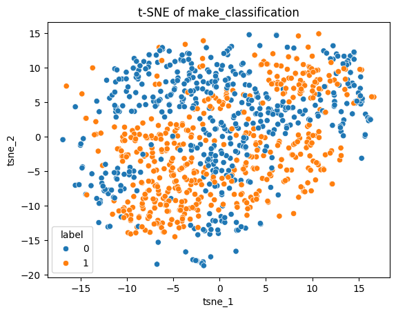

t-SNE of sklearn’s digits¶

digit_tsne = get_tsne(digit_points, log_frames=True, log_frame_interval=10)

  0%|          | 4/1000 [00:01<05:14,  3.16it/s]

100%|██████████| 1000/1000 [05:22<00:00,  3.10it/s]

plt.plot(digit_tsne["costs"])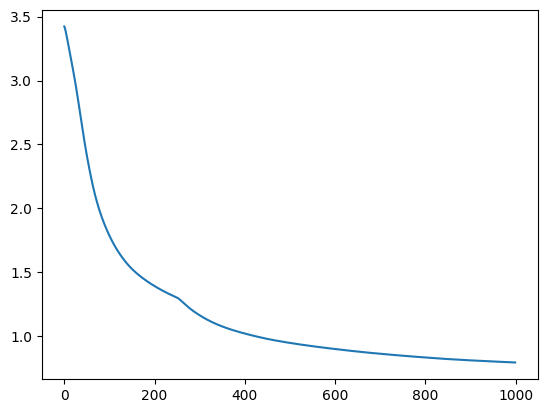

tsne_digits_df = pd.DataFrame({
    "tsne_1": digit_tsne["y_points"][:, 0],
    "tsne_2": digit_tsne["y_points"][:, 1],
    "label": digit_labels.astype(str)
})

sns.scatterplot(tsne_digits_df, x="tsne_1", y="tsne_2", hue="label")
plt.title("Digits t-SNE");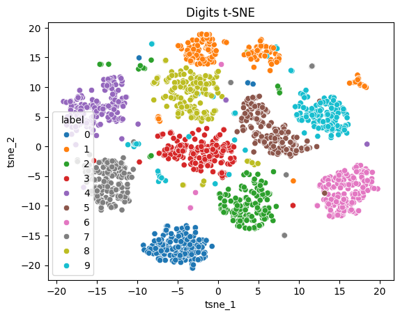

digit_frames = digit_tsne["frames"]

show_frames(digit_frames, c=digit_labels)